
Binomial Approximations
Useful ballpark estimates for almost everything

By now, you’ve probably realized that I’ve rarely dived into technical topics. The primary reason is because I believe nearly all data scientists have sufficient technical expertise to do their jobs, and also that academic and other training courses do quite well in covering technical material. The other big reason is that, most of the time, a ballpark approximation is a more judicious use of time, and just as useful as a sophisticated and precise solution (see “The Pareto Principle and Prioritization”).
To be clear, there have been many cases where having a Masters or Ph.D. in Statistics is crucial for solving certain modeling or analysis problems. The truth, though, is that even in very quantitative and data-intensive organizations, problems requiring this level of analysis or modeling complexity are in the minority of analysis needs for more generalist roles. Of course, there are specialist and frontier roles where the entire job requires extensive, deep technical expertise.
One of the jokes within the DS team is that our job consisted “most of the time adding up numbers, and if we’re especially ambitious, we’ll divide numbers.” If you’ve been reading these posts, hopefully it’s obvious that this is self-deprecating humor. Most metrics indeed are either sums (e.g., revenue) or ratios (e.g., clickthrough rate), and it’s not the arithmetical calculation that is the problems’ difficulty. Those who have done courses in Statistics also know that division, i.e., ratio metrics, can get very complicated, very fast.
I’ll admit that, after I became a manager, I spent almost zero time doing complex statistical modeling. This is both because other tasks (mostly team and cross-functional management) were much higher priority, and also because most individual contributors on the team would prefer to do such modeling rather than dealing with cross-functional stakeholders. As a data science manager, doing ballpark estimates and using heuristics (”intuition”) were the bulk of my analysis tasks.
I want to share with you some use cases of binomial approximations, and why I believe understanding the binomial distribution and its properties is extremely valuable not just for data scientists, but also for all our cross-functional partners. If you need a rough estimate of anything statistical, be it confidence intervals, significance testing, or sample size / power calculations, then binomial approximations tend to work very well for large-scale data.
Of course, there are limitations to these approximations, most commonly for rare-event or low-prevalence modeling or metrics, but also when normality assumptions don’t hold. Where binomial approximations fail just so happen to be very interesting problems for data scientists to solve. However, for most “standard” problems, a binomial approximation will generally get you the right answer within a factor of 2 or so, which is almost always good enough for these cases.
As a refresher, the binomial distribution is a discrete probability distribution that models the number of successes in a sequence of n independent trials, with each trial having a success probability p. Think of n flips of a weighted coin that comes up heads with probability p.
Its summary statistics are simple to calculate:
mean = n * p
variance = n * p * (1-p)
standard error = sqrt(p * (1-p) / n)
The binomial distribution also has a lot of nice properties. Two pertinent ones for our purposes are:
(P1) The standard error has a maximum when p = 0.5.
(P2) The binomial distribution closely approximates the normal distribution as long as n is somewhat large and p is not too close to 0 or 1.
Binomial Approximations for A/B Experiments
Using the binomial distribution for a growth metric like Daily Active Users (DAUs) in A/B experiments assumes a nonsensical model, which is that a DAU is assigned to the treatment arm with probability p and the control arm with probability 1-p. This is clearly not how user learning and growth metrics work in reality, but it’s good enough for simple approximations to more complicated calculations. Because most A/B experiments will be examining relatively modest changes in a metric, we can generally assume p = 0.5 and (P1) implies our calculations will be slightly conservative with respect to errors in this particular assumption. Of course, other assumptions might cause significant errors, but in practice we’ll be well within an order of magnitude of a more rigorous model.
For sample size calculations, we typically want to know how many observations we need to measure a particular effect size, which is generally expressed as a confidence interval half-width. An example would be: “how many DAUs do we need in each experiment arm to measure a +/-0.5% change in DAUs?”
Our binomial approximation assumes that p = 0.5 because we are looking at a small deviation from p = 0.5 in our model. A 95% confidence interval is roughly 2 * s.e. because of (P2), so the standard error s.e. = 0.5% / 2 * p = 0.00125. Solving for n:
n = p * (1-p) / (s.e.^2)
= 0.5 * 0.5 / (0.00125)^2
= 160,000
So we need around 160k DAUs in each experiment arm to measure a +/-0.5% change in DAUs. This is a very rough approximation, but I can be pretty confident that 10k is not enough, and 1M should be plenty. That’s probably all I really need to know for experiment sizing to help a team get the experiment up and running.
We can also approximately construct confidence intervals to answer questions like: “My experiment shows an increase in clicks of 0.1% from 1 million clicks in the control arm. Is that statistically significant?”
Again, assume that p = 0.5 and a 95% confidence interval is 2 * s.e. Solve for s.e.:
s.e. = sqrt(p * (1-p) / n)
= sqrt(0.5 * 0.5 / 1000000)
= 0.0005
2 * s.e. = 0.001 or 0.1%, so the 0.1% increase in clicks is likely borderline statistically significant with 95% confidence intervals.
As mentioned above, approximations for ratio metrics like clickthrough rate are more complicated and error prone, but generally speaking you can separately look at the numerator and denominator of the ratio metric to get a rough sense of experiment sizing, confidence intervals, etc. Just take these interpretations with an even larger pinch of salt.
Intuitions around Sample Sizes and Confidence Interval
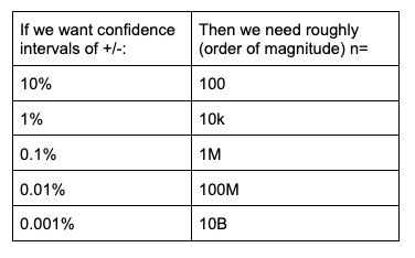
Because of the relative simplicity of the binomial distribution, it helps me with more general intuitions around mapping sample sizes and confidence intervals. For example, it’s clear from the standard error calculations above that if we want to reduce in half the confidence interval half-width (e.g., from +/- 0.2% to +/- 0.1%), we need 4x the number of observations.
Similarly, we can easily see that reducing the confidence interval half-width by an order of magnitude requires 100x the number of observations. This can be summarized as in the table below.
Stay tuned for a later post that will expound more broadly on the implications of this.